Detecting and visualizing Foobot communities with Louvain method, Spark GraphX and D3.js

Here at EnergyWise, we collect and analyze indoor pollution to make people life safer and easier.

We’re analyzing Foobot sensors data individually so we can inform and alert our customers when pollution levels are higher than recommended, but we’re also trying to analyze global trends with various technics.

Lately, we’ve been interested in using community detection algorithms. Our hopes are to analyze communities size and evolution over time, find trends, and correlate their appearance with external factors.

These algorithms are known to be used by major social networks companies to detect communities in their networks. There are also lot of academic researches in this field; analyzing various types of data sets with community detection algorithms can help find how people are connected. For instance, analyzing phone call logs can highlight where money can be invested in new infrastructure, what are the main communities in a region or country and how they are composed (among criterion like language, age, …)

There are different methods for community detection, like Minimum-cut, Hierarchical clustering, Girvan-Newman algorithm or Modularity maximization. Introductions for these methods can be found on Wikipedia

Discovering communities can also be seen as a clustering problem within graph structures.

Louvain algorithm

Louvain method was originally described¹ by Vincent D. Blondel, Jean-Loup Guillaume, Renaud Lambiotte and Etienne Lefebvre. The algorithm took the name of the Université catholique de Louvain in Belgium, where the 4 authors are researchers.

It aims at maximizing modularity using heuristic.

Definition

Modularity value to be optimized is defined as: $mod$

where

$Aij$ is the weight of the edge between i and j
$ki$ is the sum of the weights of the edges attached to i
$m$ is half the sum of all edge weights in the graph.
$ci$ is the community to which i is attached
$delta$ is 1 if $ci$ = $cj$ (same community), 0 otherwise.

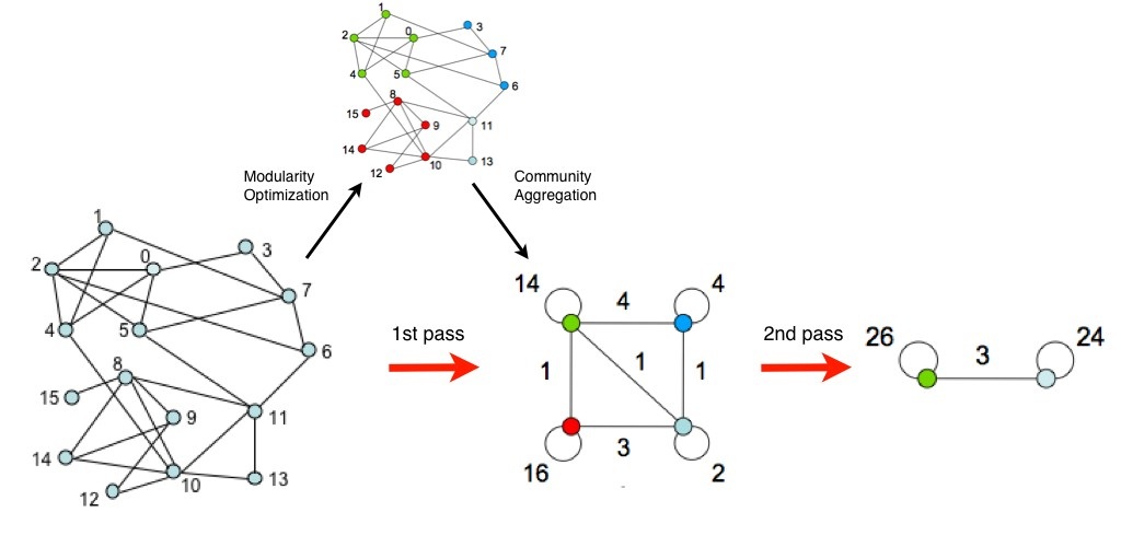
The algorithm has a 2 steps approach that are repeated iteratively until modularity value is optimized.

First, the method looks for small communities by optimizing modularity locally. Second, it aggregates nodes belonging to the same community and builds a new network. Nodes of this network are the aggregated ones built during 2nd phase. It iterates until modularity value is optimized.

A graphical representation of the iterations can be found in original paper¹, and is reproduced below

Pros

Scalability (performs faster on huge graphs than other methods)
Simple to code

Cons

Iterative process can hide small communities found during intermediate phases. The result may be a coarse-grained high level representation of communities, which may not have the granularity needed for analysis. Hopefully, the nature of the algorithm makes it simple to save intermediate phases’ results so we can analyze different communities structures at different levels
Heuristic used to initialize phases and find local maximums can lead to not reproducible and not always optimized results. But this is the same with all data algorithms relying on heuristic (K-Means² for instance)

Applications

The original study was based on phone calls logs originated from Belgian telecommunication operators.

Some public examples of applications can be found on Vincent Blondel’s personal blog.

Also, here is a detailed study made on mobile phone data sets.

An implementation for Apache Spark is available on github.

Finding Foobots communities

First of all, you may be asking: but how are Foobots connected to each other? Simple answer: they aren’t. There is no direct relation or link between 2 devices, except when they both have the same owner.

As a consequence, we will draw artificial links (or edges) between them, based on following criteria:

geographical distance³ between devices
euclidean distance⁴ between average pollutant values of devices

Same thing for edges weights: as stated in modularity definition, weight of edges is taken into account and is playing a role in nodes (or vertices) grouping.

Setting a meaningful weight on each edge is a tricky problem, and there are probably multiple solutions to it; it will highly depend on what we analyze, what we want to find or what we want to correlate to.

For the purpose of this article, we choose to define weight by using the distance between pollutant values of devices: the closer values are, the bigger weight will be.

Let’s start with fetching a Pair RDD that will have a key defined by the unique device identifier (UUID), and value being an array of the average sensor values (here taking only PM2.5⁵, although it would be interesting to include VOC⁶ too), plus geolocation of device as a (latitude, longitude) tuple. For this article, we took a sample of connected devices, and the last 30 minutes of data for each.

val loaded: RDD[(String, (Array[Double], (Double, Double)))] = ... //some function that fetches data

//(UUID, (Latitude, Longitude))
val geoList: RDD[(String,(Double,Double)] = ...

Now that we have our values, we will compute average and standard deviation for sensor values, and normalize them. Note that normalization isn’t necessary here as our input array contains only PM values.

import Utils._
val (means, stdevs) = meansAndStdevs(loaded.map(_._2._1))
val normalized = loaded
   .map {
      case (uuid, (sensorValues, geoloc)) => (uuid, (normalize(sensorValues, means, stdevs), geoloc))
}

Then we define graph vertices, by associating each UUID with a unique long identifier (from hashCode()). Long identifiers are required by Spark GraphX API.

val vertices = normalized
  .map { case (uuid, (sensorValues, geoloc)) => (uuid, (sensorValues, geoloc, uuid.hashCode().toLong)) }
  
val vertexIds: RDD[(Long, String)] = vertices.map { uuid => (uuid._2._3, uuid._1) }

Now we definie edges. We artificially link Foobots by checking their geographical distance. We define edge weight as a function of euclidean distance between 2 devices average sensor values.

val edges: RDD[Edge[Long]] = vertices
  .cartesian(vertices)
  .filter { case (uuid1, uuid2) => !uuid1._1.equals(uuid2._1) } //no loop
  .filter { case (uuid1, uuid2) => geoDistance(uuid1._2._2, uuid2._2._2) < 10 } //geo distance must be < 10km
  .map { case (uuid1, uuid2) => Edge(uuid1._2._3, uuid2._2._3, (1/euclideanDistance(uuid1._2._1, uuid2._2._1)).toLong) }

And then, we generate the graph:

val graph = Graph(vertexIds, edges)

Now that we have a graph, we can run Louvain algorithm on it. Our reference implementation can be found here. We slightly modified it, mainly to keep stages data in memory so we don’t require HDFS.

val runner = new InMemoryLouvainRunner(5, 3)
val louvainGraph: Graph[VertexState, Long] = runner.run(sc, graph)

Time for a little reverse mapping game: remember we mapped UUIDs with Long identifiers. We want to get UUIDs back. We then map each vertex id in edges (source and destination) with their corresponding UUID.

val resolvedEdges = louvainGraph.edges
  .map { edge => (edge.srcId, (edge.dstId, edge.attr)) }
  .join(vertexIds)
  .map { case (vxSrcId, ((vxDstId, linkWeight), srcUuid)) => (vxDstId, (linkWeight, srcUuid)) }
  .join(vertexIds)
  .map { case (vxDstId, ((linkWeight, srcUuid), dstUuid)) => (srcUuid, dstUuid, linkWeight) }

Here is the final step: output the result as a JSON file that will be used later to plot our results in graphs.

//Helper classes
case class JsNode(name: String, communityId: Int, value: Int, polLevel: Double)
case class JsLink(source: Int, target: Int, value: Int)
case class JsGraph(nodes: Array[JsNode], links: Array[JsLink])

//Transform vertices
val geoNodes: Array[JsNode] = resolvedVertices
  .join(geoList)
  .map {
     case (uuid, (state, (lat, lon))) =>
       val (strLat, strLon) = strLoc(lat, lon)
       (uuid, (strLat, strLon, scaledWeight(state.nodeWeight)))
  }
  .join(loaded)
  .map { case (uuid, ((strLat, strLon, weight), ((values, loc)))) => (uuid.hashCode().toInt, strLat, strLon, weight, values(0)) }
  .map { geoNode => JsNode(s"${geoNode._2} ${geoNode._3}", geoNode._1, geoNode._4.toInt, geoNode._5) }
  .distinct()
  .collect()

//Transform edges
val jsonEdges: Array[JsLink] = louvainGraph.edges
  .map { edge => JsLink(edge.srcId.toInt, edge.dstId.toInt, scaledWeight(edge.attr).toInt) }
  .collect()

//Output to file
mapper.writeValue(new File("/var/www/html/communities.json"), JsGraph(geoNodes, jsonEdges))

Plotting results with D3

Let’s plot our results to visualize more clearly size of communities and links between them. Here we use D3.js for the tons of features and graph types it provides, and first graph we plot is a Force directed graph (definition and other exemples here)

This gives us a first overview of how communities were built, and how they are “linked”. Note that size of node is given by community weight, but this weight has been scaled (logarithmically) so it can fit on a map. So are much bigger than what is actually rendered.

Finally, as we have kept geographical coordinates of communities (by assigning one of the Foobot’s to the community – could be more accurate by taking the one which has the smaller distance to every other), it is possible to plot a map, like below.

Notes:

Data snapshot at 2016-02-09 4.PM GMT (11.AM EST / 8.AM PST)

Summary

In this article we’ve seen an introduction on communities detection in graphs, especially with Louvain algorithm, and we’ve used Foobot dataset to compute and plot communities on a map. Deeper investigation could include:

try another algorithm, like DBSCAN
find how communities come and go, analyze and predict appearance of population of users with bad air quality.
study correlation with external factors, like outdoor air quality.